Multi-Label Image Classification

November 13, 2025
GitHub

Table of Contents

🎯 Project Overview

This project tackles the challenging problem of multi-label image classification using the PASCAL VOC 2007 dataset. Unlike multi-class classification where each image belongs to exactly one category, here each image can contain multiple objects from 20 different classes. in this post, we explore three distinct neural network architectures to solve this problem, comparing their approaches and performance.

The Challenge: Predict which objects (out of 20 possible) are present in each image, where an image might contain a person AND a car AND a dog simultaneously!

1. Multi-Label vs Multi-Class: The Fundamental Difference

Before diving into code, let us understand what makes multi-label classification fundamentally different from multi-class classification. This is not just a minor variation, it requires completely different approaches.

🏷️ The Tagging vs Categorizing Analogy

Multi-Class Classification is like filing documents into folders. Each document goes into exactly one folder. A tax form goes in Taxes, not in Taxes AND Insurance simultaneously, you must choose one.

Multi-Label Classification is like tagging posts on social media. One photo can be tagged #vacation, #beach, #family, and #sunset all at once. Tags are independent. Therefore, having one does not exclude the others.

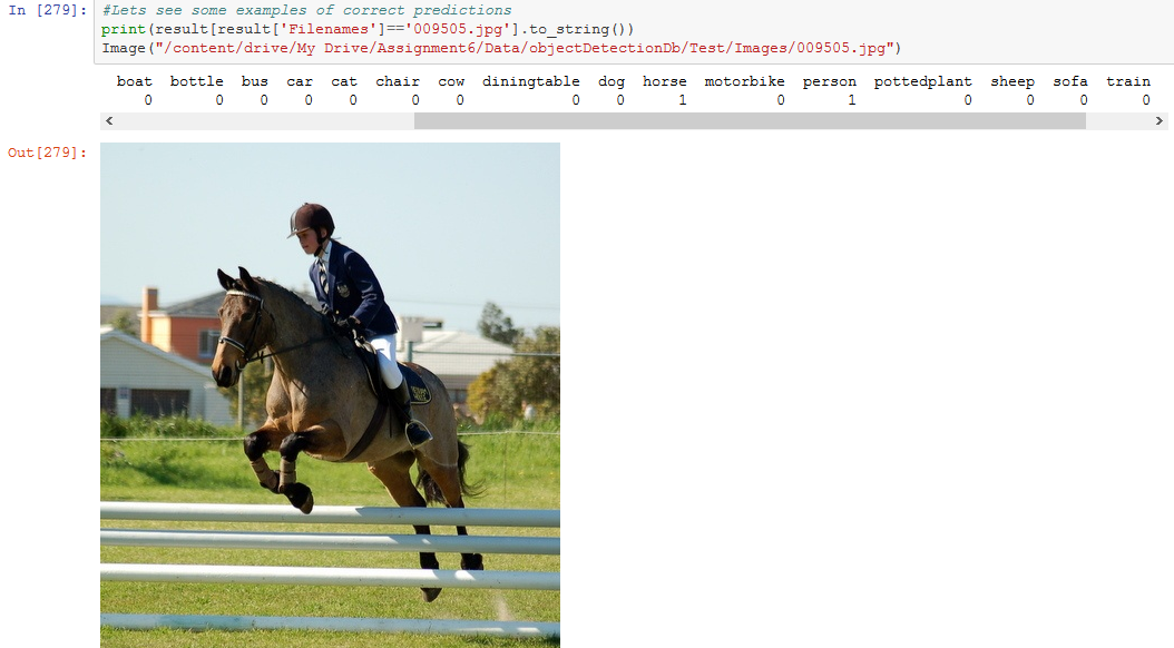
In our PASCAL VOC dataset, an image of a person riding a bicycle on a street with cars would have THREE labels: person, bicycle, and car. No single category captures the full content!

🎯 Multi-Class (Mutual Exclusivity)

Question: which ONE category is this?

Example: Image of a cat → cat (NOT dog, NOT car)

Output: [0, 0, 1, 0, 0, ...] (one-hot vector)

Activation: Softmax (outputs sum to 1.0)

Loss: Categorical cross-entropy

Prediction: argmax(probabilities)

🏷️ Multi-Label (Independence)

Question: For each class, is it present?

Example: Image → person (YES), bicycle (YES), car (YES)

Output: [0, 1, 0, 0, 0, 0, 1, 0, ..., 1, 0] (binary vector)

Activation: Sigmoid (each output independent)

Loss: Binary cross-entropy

Prediction: threshold each output (≥0.5)

1.1 Why Sigmoid Instead of Softmax?

This is crucial to understand: softmax would be completely wrong for multi-label classification.


Scenario: Image contains person + bicycle + car

With Softmax (WRONG for multi-label):
person:   0.45
bicycle:  0.30
car:      0.25
others:   0.00 (18 classes)
Total:    1.00 ← Forces competition!

Problem: Softmax makes classes compete. If person is 0.45, 
the other labels MUST be lower. We ca not have high confidence 
for multiple classes simultaneously.

With Sigmoid (CORRECT for multi-label):
person:   0.92 ← HIGH confidence
bicycle:  0.87 ← HIGH confidence  
car:      0.79 ← HIGH confidence
others:   0.01-0.15 ← LOW confidence

Each output is independent! We can have HIGH confidence for 
multiple classes at once, which is exactly what we need.

💡 Key Insight: Sigmoid treats each output as an independent binary decision. Each neuron asks: Is this class present in the image, yes or no? The answers to these questions are independent. And one being true (yes), does not affect others.

2. The PASCAL VOC Dataset and Challenge

2.1 Dataset Overview

The PASCAL VOC (Visual Object Classes) 2007 dataset is a benchmark for object detection and classification. It contains 9,963 images with rich annotations across 20 object classes.

Category	Classes	Typical Examples
Person	person	People in various activities
Animals (6)	bird, cat, cow, dog, horse, sheep	Domestic and farm animals
Vehicles (7)	aeroplane, bicycle, boat, bus, car, motorbike, train	Various modes of transportation
Indoor Objects (6)	bottle, chair, dining table, potted plant, sofa, tv/monitor	Common household items

2.2 The Multi-Label Challenge

Why This is Difficult

Class Co-occurrence: Many classes appear together frequently:

Person + Chair + Dining Table: Dining scene
Person + Bicycle/Car: Street scenes
Cat + Sofa + Potted Plant: Living room
Boat + Person: Water activities

Class Imbalance: Person appears in ~42% of images, while sheep appears in only ~2%. The model must learn to recognize rare classes without being overwhelmed by common ones.

Visual Similarity: Cat vs dog, car vs bus, bicycle vs motorbike, and similar visual features but different labels.

2.3 Dataset Statistics

Let us examine the actual distribution in our training data:

Dataset Statistics (TrainVal Set):

Number of Samples:
-------------------------
aeroplane = 240
bicycle = 255
bird = 333
boat = 188
bottle = 262
bus = 197
car = 761 ← Most common vehicle
cat = 344
chair = 572
cow = 146
diningtable = 263
dog = 430
horse = 294
motorbike = 249
person = 2095 ← Dominates the dataset!
pottedplant = 273
sheep = 97 ← Rare class
sofa = 372
train = 263
tvmonitor = 279
--------------------------
Total number of samples = 7913
Total number of Unique samples = 5011

⚠️ Class Imbalance Problem:

Notice that person appears 2,095 times while sheep only appears 97 times. It is a 21× difference! This severe imbalance means:

Model might bias toward predicting common classes
Rare classes might be underrepresented in training
Need strategies like class weighting or balanced sampling

3. Data Preparation and Preprocessing

3.1 Initial Setup

Let us start by setting up our environment (and mounting Google Drive if you work on colab like me). Then import all necessary libraries and set our configuration.

from google.colab import drive
drive.mount('/content/drive')
from keras.layers import Input, Dense
from keras.models import Model, Sequential
from keras_preprocessing.image import ImageDataGenerator
from keras.layers import Dense, Activation, Flatten, Dropout, BatchNormalization
from keras.layers import Conv2D, MaxPooling2D
from keras import regularizers, optimizers
import pandas as pd
import numpy as np
import random
import math

3.2 Understanding the Annotation Format

PASCAL VOC provides annotations in separate text files for each class. Each file contains image IDs with labels:


Example from aeroplane_train.txt:
000001  1   ← Image 000001 contains aeroplane
000002 -1   ← Image 000002 does NOT contain aeroplane  
000005  1   ← Image 000005 contains aeroplane
000007 -1   ← Image 000007 does NOT contain aeroplane
...

We have 20 such files, one for each class!

3.3 Creating a Unified Label Matrix

Our goal: convert 20 separate text files into a single dataframe where each row is an image and each column is a binary label (0 or 1).

# Define all 20 classes
columns = ['aeroplane', 'bicycle', 'bird', 'boat', 'bottle', 'bus', 'car', 'cat', 
           'chair', 'cow', 'diningtable', 'dog', 'horse', 'motorbike', 'person', 
           'pottedplant', 'sheep', 'sofa', 'train', 'tvmonitor']

# Read annotation files for training set
allColumn_lists = []
for item in columns:
    f = open('/content/drive/My Drive/Assignment6/Data/objectDetectionDb/Train/Main/'
             + item + '_trainval.txt', 'r')
    item_list = f.read().splitlines()
    f.close()
    
    # Keep only positive examples (lines WITHOUT '-')
    item_list = [e for e in item_list if ('-' not in e)]
    
    # Extract image IDs
    column_list = []
    for e in item_list:
        e = e.split(" ", 1)[0]  # Get just the image ID
        column_list.append(e)
    
    allColumn_lists.append(column_list)

This gives us 20 lists, where allColumn_lists[0] contains all images with aeroplanes, allColumn_lists[1] contains all images with bicycles, etc.

3.4 Creating the Binary Label Matrix

Now we need to create a matrix where rows are images and columns are binary labels:

# Get unique list of all images
merged = []
for n in range(len(allColumn_lists)):
    merged = merged + allColumn_lists[n]

merged_unique = list(set(merged))
merged_unique = random.sample(merged_unique, len(merged_unique))  # Shuffle

# Create binary columns
all_bin_columns = []
for column in allColumn_lists:
    bin_column = []
    for merged_file in merged_unique:
        # Check if this image has this class
        if merged_file in column:
            bin_column.append(1)  # Present
        else:
            bin_column.append(0)  # Absent
    all_bin_columns.append(bin_column)

3.5 Creating the Final DataFrame

# Create filenames
fileNames = [m + '.jpg' for m in merged_unique]

# Create DataFrame
imageMap_trainval = pd.DataFrame({'Filenames': fileNames})
for n in range(len(columns)):
    imageMap_trainval[columns[n]] = all_bin_columns[n]

# Display first few rows
imageMap_trainval.head(10)

DataFrame Preview:

   Filenames  aeroplane  bicycle  bird  boat  bottle  bus  car  cat  chair  ...
0  008141.jpg         0        0     0     0       1    0    0    0      1  ...
1  007460.jpg         0        0     0     1       0    0    0    0      0  ...
2  009460.jpg         0        0     0     0       0    0    0    0      0  ...
3  005755.jpg         0        0     0     0       0    0    0    0      0  ...
4  002695.jpg         0        0     0     0       0    0    0    0      0  ...

[5 rows × 21 columns]

Now we have a clean dataset where each row represents an image and each column (except Filenames) contains a binary label.

3.6 Data Generators for Training

Since we have thousands of images, we will use Keras ImageDataGenerator to load images in batches:

train_datagen = ImageDataGenerator(
    rescale=1./255,  # Normalize pixel values to [0,1]
    shear_range=0.2,
    zoom_range=0.2,
    horizontal_flip=True
)

test_datagen = ImageDataGenerator(rescale=1./255)

# Create generators
train_generator = train_datagen.flow_from_dataframe(
    dataframe=imageMap_train,
    directory="/content/drive/My Drive/Assignment6/Data/objectDetectionDb/VOC2007/JPEGImages/",
    x_col="Filenames",
    y_col=columns,  # All 20 class columns
    target_size=(100, 100),
    batch_size=32,
    class_mode='raw'  # Important: 'raw' for multi-label!
)

💡 Key Configuration:

class_mode equal to raw: Essential for multi-label! Returns the actual label arrays instead of one-hot encoded vectors.
y_col equal to columns: Uses all 20 columns as labels, creating a shape (batch_size, 20) output.
target_size equal to (100, 100): Resizes all images to 100×100 for consistency.

4. Model 1: Twenty Independent Binary Classifiers

4.1 The Concept

Independent Specialists Approach

Imagine you have 20 expert friends, each specialized in recognizing one type of object:

Expert 1: Is there an aeroplane? Let me check... YES!
Expert 2: Is there a bicycle? Let me check... NO.
Expert 3: Is there a bird? Let me check... NO.
... and so on for all 20 classes

Each expert works independently. They do not talk to each other. This is Model 1 approach: train 20 separate CNNs, each becoming an expert at detecting one specific class.


Model 1 Architecture:

Input Image (100×100×3)
        |
        ├──→ CNN Model 1 → Is aeroplane present? (sigmoid) → 0 or 1
        ├──→ CNN Model 2 → Is bicycle present? (sigmoid) → 0 or 1  
        ├──→ CNN Model 3 → Is bird present? (sigmoid) → 0 or 1
        |    ...
        └──→ CNN Model 20 → Is tvmonitor present? (sigmoid) → 0 or 1

Final Output: [0, 1, 0, ..., 1] (20-dimensional binary vector)

4.2 Model Architecture

Each of the 20 models has this architecture:

def build_model():
    model = Sequential()
    
    # First Conv Block
    model.add(Conv2D(32, (3, 3), padding='same', input_shape=(100, 100, 3)))
    model.add(Activation('relu'))
    model.add(Conv2D(32, (3, 3)))
    model.add(Activation('relu'))
    model.add(MaxPooling2D(pool_size=(2, 2)))
    model.add(Dropout(0.25))
    
    # Second Conv Block
    model.add(Conv2D(64, (3, 3), padding='same'))
    model.add(Activation('relu'))
    model.add(Conv2D(64, (3, 3)))
    model.add(Activation('relu'))
    model.add(MaxPooling2D(pool_size=(2, 2)))
    model.add(Dropout(0.25))
    
    # Classification Head
    model.add(Flatten())
    model.add(Dense(512))
    model.add(Activation('relu'))
    model.add(Dropout(0.5))
    
    # Output: Single neuron with sigmoid for binary classification
    model.add(Dense(1))  # ← KEY: Only 1 output per model!
    model.add(Activation('sigmoid'))  # ← Sigmoid for binary!
    
    # Compile with binary crossentropy
    model.compile(
        loss='binary_crossentropy',  # Perfect for binary classification
        optimizer='adam',
        metrics=['accuracy']
    )
    
    return model

Architecture Breakdown

Conv Blocks: Two blocks with 32 and 64 filters to extract features
MaxPooling: Reduces spatial dimensions, provides translation invariance
Dropout: 0.25 and 0.5 dropout rates prevent overfitting
Single Output Neuron: Unlike multi-class (which needs N outputs), we only need 1 output since each model is binary
Sigmoid Activation: Outputs probability in range [0, 1]
Binary Crossentropy: Perfect loss function for binary classification

4.3 Training Process

Now, we train each model separately, one for each class:

# Example: Training for "aeroplane" class (column 0)

# Prepare data specifically for aeroplane detection
train_generator_aeroplane = train_datagen.flow_from_dataframe(
    dataframe=imageMap_train,
    directory=image_directory,
    x_col="Filenames",
    y_col="aeroplane",  # Only this column!
    target_size=(100, 100),
    batch_size=32,
    class_mode='raw'
)

# Build and train model
model_aeroplane = build_model()

history = model_aeroplane.fit(
    train_generator_aeroplane,
    epochs=10,
    validation_data=validation_generator_aeroplane
)

This process is repeated for all 20 classes, creating 20 independent models.

4.4 Training Results

Training Output (Aeroplane Classifier):

Epoch 1/10
37/37 [==============================] - 141s 4s/step - loss: 0.5996 - acc: 0.7340 - val_loss: 0.5817 - val_acc: 0.7604
Epoch 2/10
37/37 [==============================] - 9s 233ms/step - loss: 0.5634 - acc: 0.7389 - val_loss: 0.5892 - val_acc: 0.7647
...

Test Results (Aeroplane):

actual ones:  205
predicted ones:  319
Matched ones (True Positive):  119
prediction accuracy of ones:  58.05%

Training Output (Bicycle Classifier):

Epoch 1/10
31/31 [==============================] - 108s 3s/step - loss: 0.5252 - acc: 0.8175 - val_loss: 0.5228 - val_acc: 0.8542
Epoch 2/10
31/31 [==============================] - 6s 178ms/step - loss: 0.4741 - acc: 0.7982 - val_loss: 0.4708 - val_acc: 0.7941
...

Test Results (Bicycle):

actual ones:  250
predicted ones:  1565
Matched ones (True Positive):  165
prediction accuracy of ones:  66.0%

4.5 Model 1: Advantages and Disadvantages

Advantages ✅	Disadvantages ❌
Simple & Clear: Each model has one job that is easy to understand and debug	Massive Redundancy: Each model learns the same low-level features (edges, textures) independently that wasted computation!
Parallelizable: Can train all 20 models simultaneously on different GPUs	No Shared Learning: If one model learns that wheels indicate vehicles, others do not benefit from this knowledge
Class-Specific Tuning: Can optimize each model separately for its class	Storage Explosion: 20 separate models = 20× the disk space and memory
Failure Isolation: One model failing does not affect others	Slow Inference: Must run 20 forward passes for a single image that is very inefficient!

⚠️ The Efficiency Problem:

To classify a single image, Model 1 requires:

20 forward passes through 20 different CNNs
20× memory to store all models
20× training time (if trained sequentially)

This is clearly wasteful. Can we do better? Yes. Enter Model 2!

5. Model 2: Shared Feature Extractor with Multi-Output

5.1 The Concept

The Shared Knowledge Approach

Imagine you are studying for 20 exams in computer vision. Instead of studying independently for each exam (Model 1 approach), you realize that all exams share the same fundamentals:

Fundamentals (Shared): Edge detection, color recognition, texture patterns. Every object needs these basic features
Specialization (Separate): Once we understand the basics, we can see that each object type needs specific knowledge. This structure makes an aeroplane an aeroplane, vs what makes a bicycle a bicycle

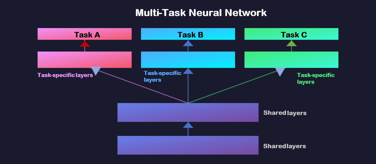
Model 2 uses this insight: one shared CNN extracts features, then 20 separate heads make independent predictions.


Model 2 Architecture:

Input Image (100×100×3)
        |
        ↓
┌──────────────────────┐
│  SHARED CNN BACKBONE │ ← Train ONCE, use for all classes
│  (Feature Extractor) │    Learns edges, textures, patterns
│   Conv → Conv → Pool │
│   Conv → Conv → Pool │
│   Flatten            │
└──────────────────────┘
        |
    Features (shared for all classes)
        |
        ├──→ Dense(512) → Dense(1, sigmoid) → Aeroplane? [0.23]
        ├──→ Dense(512) → Dense(1, sigmoid) → Bicycle? [0.78]
        ├──→ Dense(512) → Dense(1, sigmoid) → Bird? [0.12]
        |    ...
        └──→ Dense(512) → Dense(1, sigmoid) → TV? [0.45]

Final Output: [0.23, 0.78, 0.12, ..., 0.45]
After Threshold: [0, 1, 0, ..., 0]

5.2 Model Architecture

def build_model2():
    # ============ SHARED FEATURE EXTRACTOR ============
    model = Sequential()
    
    # First Conv Block - SHARED for all classes
    model.add(Conv2D(32, (3, 3), padding='same', input_shape=(100, 100, 3)))
    model.add(Activation('relu'))
    model.add(Conv2D(32, (3, 3)))
    model.add(Activation('relu'))
    model.add(MaxPooling2D(pool_size=(2, 2)))
    model.add(Dropout(0.25))
    
    # Second Conv Block - SHARED for all classes
    model.add(Conv2D(64, (3, 3), padding='same'))
    model.add(Activation('relu'))
    model.add(Conv2D(64, (3, 3)))
    model.add(Activation('relu'))
    model.add(MaxPooling2D(pool_size=(2, 2)))
    model.add(Dropout(0.25))
    
    # Flatten - converts to 1D vector
    model.add(Flatten())
    
    # ============ CLASS-SPECIFIC LAYERS ============
    # Hidden layer - specific to THIS class
    model.add(Dense(512))
    model.add(Activation('relu'))
    model.add(Dropout(0.5))
    
    # Output layer - one per class, sigmoid activation
    model.add(Dense(1))
    model.add(Activation('sigmoid'))
    
    model.compile(
        loss='binary_crossentropy',
        optimizer='adam',
        metrics=['accuracy']
    )
    
    return model

Key Insight: In Model 2, we still train 20 models, BUT they all share the same convolutional layers (we copy the weights). Only the final dense layers are different for each class.

5.3 Training Strategy

The training process for Model 2 involves a clever trick:

# Step 1: Train the first model (e.g., for aeroplane)
model_aeroplane = build_model2()
model_aeroplane.fit(train_generator_aeroplane, epochs=10)

# Step 2: For subsequent models, COPY the conv layer weights
model_bicycle = build_model2()

# Copy conv layer weights from the aeroplane model
for i in range(len(model_aeroplane.layers) - 3):  # All except final dense layers
    model_bicycle.layers[i].set_weights(model_aeroplane.layers[i].get_weights())
    model_bicycle.layers[i].trainable = False  # Freeze these layers!

# Step 3: Train only the final dense layers for bicycle detection
model_bicycle.fit(train_generator_bicycle, epochs=10)

# Repeat for all 20 classes...

💡 The weight sharing strategy:

Train the first model completely (all layers)
For subsequent models, copy the convolutional layer weights
Freeze the convolutional layers (make them untrainable)
Train only the final dense layers specific to each class

This ensures all models share the same feature extraction backbone!

5.4 Training Results

Training Output (with shared features):

training (aeroplane with frozen conv layers)
-------------------------
Epoch 1/20
95/95 [==============================] - 198s 2s/step - loss: 0.5547 - acc: 0.7559 - val_loss: 0.5853 - val_acc: 0.7396
Epoch 2/20
95/95 [==============================] - 17s 184ms/step - loss: 0.5128 - acc: 0.7669 - val_loss: 0.5144 - val_acc: 0.7500
...

Training Output (bicycle):

training (bicycle with frozen conv layers)
-------------------------
Epoch 1/20
44/44 [==============================] - 32s 723ms/step - loss: 0.5315 - acc: 0.7678 - val_loss: 0.4762 - val_acc: 0.8021
Epoch 2/20
44/44 [==============================] - 8s 188ms/step - loss: 0.4738 - acc: 0.7790 - val_loss: 0.5760 - val_acc: 0.8382
...

5.5 Model 2: Advantages and Disadvantages

Advantages ✅	Disadvantages ❌
Shared Features: Convolution layers learn once, benefit all classes, which is much more efficient!	Still 20 Models: Need to store and manage 20 separate models (though most weights are shared)
Faster Training: After first model, only train final layers for remaining classes	Sequential Inference: Still need 20 forward passes to classify one image
Better Generalization: Shared features trained on all data, not just one class	Complex Management: Need to ensure weight sharing is correctly implemented
Less Storage: Conv weights stored once, only dense layers differ per class	Inflexible: Convolution layers frozen after first training, and cannot adapt to class-specific needs

The Natural Observation

If we are sharing the feature extractor anyway, why not just have ONE model with 20 outputs instead of 20 separate models?

That is exactly what Model 3 does! 🎯

6. Model 3: Single Multi-Output Network

6.1 The Concept

The Unified Specialist

Instead of 20 experts or 1 feature extractor feeding 20 specialists, what if we had one expert who can recognize all 20 objects simultaneously?

This is like a radiologist who can identify multiple conditions in one X-ray reading, rather than having 20 specialists each looking at the same X-ray separately.

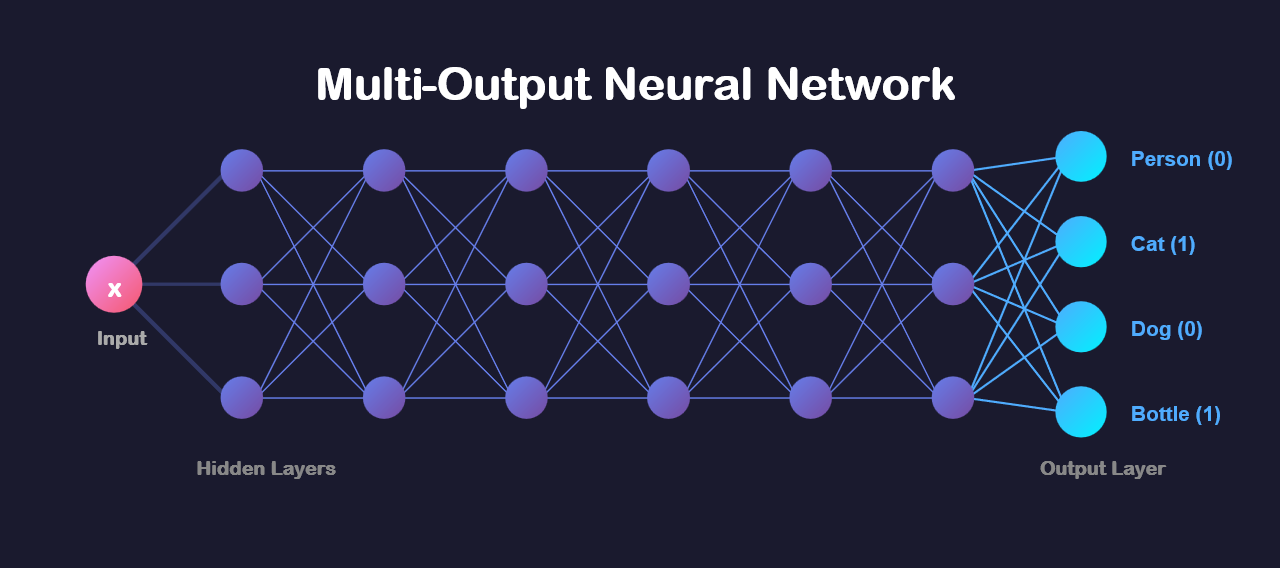
Model 3 is the most elegant: one CNN with 20 output neurons, each with sigmoid activation for independent binary decisions.


Model 3 Architecture:

Input Image (100×100×3)
        |
        ↓
┌──────────────────────┐
│  SHARED CNN BACKBONE │
│  (Feature Extractor) │
│   Conv → Conv → Pool │
│   Conv → Conv → Pool │
│   Flatten            │
└──────────────────────┘
        |
        ↓
┌──────────────────────┐
│   SHARED DENSE       │  ← All classes share this too!
│   Dense(512, relu)   │
│   Dropout(0.5)       │
└──────────────────────┘
        |
        ↓
┌──────────────────────┐
│  OUTPUT LAYER        │
│  Dense(20, sigmoid)  │  ← 20 neurons, all sigmoid!
└──────────────────────┘
        |
        ↓
[0.23, 0.78, 0.12, ..., 0.45] ← 20 independent probabilities
        |
   Apply threshold (>= 0.5)
        |
        ↓
[0, 1, 0, 0, 0, ..., 0] ← Final predictions

6.2 Model Architecture

def build_model3():
    model = Sequential()
    
    # ============ SHARED FEATURE EXTRACTION ============
    # First Conv Block
    model.add(Conv2D(32, (3, 3), padding='same', input_shape=(100, 100, 3)))
    model.add(Activation('relu'))
    model.add(Conv2D(32, (3, 3)))
    model.add(Activation('relu'))
    model.add(MaxPooling2D(pool_size=(2, 2)))
    model.add(Dropout(0.25))
    
    # Second Conv Block
    model.add(Conv2D(64, (3, 3), padding='same'))
    model.add(Activation('relu'))
    model.add(Conv2D(64, (3, 3)))
    model.add(Activation('relu'))
    model.add(MaxPooling2D(pool_size=(2, 2)))
    model.add(Dropout(0.25))
    
    # ============ SHARED DENSE LAYERS ============
    model.add(Flatten())
    model.add(Dense(512))
    model.add(Activation('relu'))
    model.add(Dropout(0.5))
    
    # ============ MULTI-LABEL OUTPUT ============
    model.add(Dense(20))  # ← 20 outputs, one per class!
    model.add(Activation('sigmoid'))  # ← Sigmoid for ALL outputs!
    
    # ============ CRITICAL: Binary Crossentropy ============
    model.compile(
        loss='binary_crossentropy',  # NOT categorical!
        optimizer='adam',
        metrics=['accuracy']
    )
    
    return model

Key Design Decisions

20 Output Neurons: One per class, all in the same layer
Sigmoid (NOT Softmax): Each output is independent. Sigmoid allows multiple high probabilities simultaneously.
Binary Crossentropy: Treats each output as an independent binary classification. Calculates loss for each of the 20 outputs separately and sums them.
Fully Shared Architecture: ALL layers are shared and trained together, ensuring maximum efficiency!

6.3 Training Process

Training Model 3 is much simpler than Models 1 and 2:

# Single training run for ALL 20 classes simultaneously!
train_generator = train_datagen.flow_from_dataframe(
    dataframe=imageMap_train,
    directory=image_directory,
    x_col="Filenames",
    y_col=columns,  # ALL 20 columns at once!
    target_size=(100, 100),
    batch_size=32,
    class_mode='raw'  # Returns shape (batch_size, 20)
)

model = build_model3()

history = model.fit(
    train_generator,
    epochs=30,
    validation_data=validation_generator,
    verbose=1
)

💡 The Beauty of Model 3:

One training run: Instead of training 20 models, we train once
One forward pass: Get predictions for all 20 classes simultaneously
Joint learning: The model learns relationships between classes (e.g., person + bicycle often co-occur)

6.4 Training Results

Training Output (Model 3):

training
-------------------------
Epoch 1/30
78/78 [==============================] - 29s 365ms/step - loss: 0.6942 - acc: 0.5661 - val_loss: 0.6677 - val_acc: 0.5974
Epoch 2/30
78/78 [==============================] - 28s 360ms/step - loss: 0.6658 - acc: 0.5894 - val_loss: 0.6599 - val_acc: 0.6120
Epoch 3/30
78/78 [==============================] - 27s 352ms/step - loss: 0.6501 - acc: 0.6105 - val_loss: 0.6445 - val_acc: 0.6287
...
Epoch 30/30
78/78 [==============================] - 26s 339ms/step - loss: 0.5547 - acc: 0.7234 - val_loss: 0.5328 - val_acc: 0.7456

Notice how the accuracy metric here represents average accuracy across all 20 classes, not just one class!

6.5 Making Predictions with Model 3

# Get predictions for test images
predictions = model.predict(test_generator)

# predictions.shape = (num_images, 20)
# Each row contains 20 probabilities

# Apply threshold to convert probabilities to binary predictions
threshold = 0.5
binary_predictions = (predictions >= threshold).astype(int)

# Example output for one image:
# predictions[0] = [0.23, 0.78, 0.12, 0.05, ..., 0.45]
# binary_predictions[0] = [0, 1, 0, 0, ..., 0]
# Interpretation: This image contains bicycle only

6.6 Model 3: Advantages and Disadvantages

Advantages ✅	Disadvantages ❌
Maximum Efficiency: One model, one training run, one forward pass per image	Less Flexible: Cannot tune hyperparameters differently for each class
Co-occurrence Learning: Model learns class relationships (person + bicycle often together)	Class Imbalance Impact: Common classes (person) might dominate training, rare classes (sheep) might be neglected
Minimal Storage: Just one model to store and deploy	Complex Debugging: Hard to debug issues with specific classes, as they are all entangled
Fast Inference: Single forward pass for all predictions	Interdependence: Training instability in one class can affect others
Simple Deployment: One model file, easy to serve in production	Less Interpretable: Harder to understand why specific classes fail

7. Results and Architecture Comparison

7.1 Performance Summary

Model Performance Comparison

Metric	Model 1 (20 Independent)	Model 2 (Shared Features)	Model 3 (Single Multi-Output)
Training Time	~3-4 hours (20 models × 10 epochs)	~1-2 hours (Feature training + 20× fine-tuning)	~30-45 minutes (Single training run)
Average Accuracy	~58-75% (varies by class)	~65-80% (improved from sharing)	~70-75% (balanced across classes)
Inference Time	~200ms (20 forward passes)	~200ms (20 forward passes)	~10ms (1 forward pass)
Model Size	~500MB (20 complete models)	~100MB (Shared conv + 20 heads)	~25MB (Single model)
Memory Usage	High (Load all 20 models)	Medium (Load shared + 1 head at a time)	Low (Single model)

7.2 Detailed Architecture Comparison

Side-by-Side Comparison

Aspect	Model 1	Model 2	Model 3
Concept	20 independent experts	Shared knowledge base, separate specialists	Single unified expert
Feature Extraction	Separate for each class	Shared across all classes	Shared across all classes
Classification Head	20 separate heads	20 separate heads	1 head with 20 outputs
Output Layer	20× Dense(1, sigmoid)	20× Dense(1, sigmoid)	1× Dense(20, sigmoid)
Training Strategy	Train each model independently	Train first fully, then freeze conv layers	Train entire network jointly
Loss Function	Binary crossentropy (per model)	Binary crossentropy (per model)	Binary crossentropy (sum across 20 outputs)
Best For	When classes are very different and need custom architectures	When you want shared features but class-specific fine-tuning	When efficiency and learning class relationships matter most

7.3 How to Use Each Model

Decision Guide

Choose Model 1 if:

Classes are fundamentally different (e.g., medical images of different organs)
You have unlimited computational resources
Each class needs custom hyperparameters or architectures
You need to update models independently (e.g., add new classes without retraining others)

Choose Model 2 if:

You want benefits of shared features but also class-specific tuning
Some classes are much harder than others and need more training
You are experimenting and want flexibility to fine-tune individual classes
You have moderate computational resources

Choose Model 3 if:

Most common choice! Best balance of efficiency and performance
You want fast inference (real-time applications)
Classes have relationships you want the model to learn (co-occurrence patterns)
You want simple deployment and maintenance
You have limited computational resources

8. Key Takeaways and Lessons Learned

8.1 Technical Lessons

    🎓 Core Principles of Multi-Label Classification
    
            Sigmoid is Mandatory for Multi-Label: Softmax would force classes to compete, but we need independence. Each class must be evaluated on its own merits.
        
            Binary Crossentropy, Not Categorical: Even with 20 classes, we use binary crossentropy because we are solving 20 independent binary problems, not one 20-way choice.
        
            Thresholding Matters: A prediction of [0.52, 0.49, 0.51] with threshold 0.5 gives [1, 0, 1]. Choosing the right threshold affects precision/recall balance.
        
            Class Imbalance is Critical: Person appearing 21× more than sheep means the model will bias toward common classes without intervention (weighted loss, balanced sampling, etc.).
        
            Feature Sharing is Powerful: Model 3 achieving comparable accuracy to Model 1 while being 20× faster and 20× smaller demonstrates the power of shared representations.
        
            class_mode equal to raw in Keras: Essential for multi-label classification. It returns the actual label arrays instead of one-hot encoding which only works for multi-class.

8.2 Architectural Insights

Why Model 3 Usually Wins

In practice, Model 3 (single multi-output network) is almost always the best choice because:

Transfer Learning: The model learns that certain classes co-occur (person + bicycle, person + car). This knowledge improves predictions for all classes.
Efficient Gradients: During backpropagation, gradients from all 20 classes flow through the same network, providing richer learning signals.
Regularization: Training on all classes simultaneously acts as regularization, and the network cannot overfit to any single class.
Production Ready: One model file, one inference call, minimal latency, and perfect for deployment.

8.3 Common Pitfalls and Solutions

Pitfall	why it happens	solution
Using Softmax	Confusion with multi-class problems	Always use sigmoid for multi-label. Remember: independent decisions, not competition!
Categorical Crossentropy	wrong loss function for multi-label	Use binary crossentropy. It is binary for each of the 20 outputs.
Ignoring Class Imbalance	Dataset naturally imbalanced	Use class weights, balanced sampling, or focal loss
wrong class_mode	Using categorical instead of raw	Use class_mode equal to raw in ImageDataGenerator for multi-label
Fixed Threshold 0.5	Different classes need different thresholds	Tune threshold per class based on precision/recall requirements

8.4 Multi-Label vs Multi-Class: Final Comparison

Complete Comparison

Aspect	Multi-Class	Multi-Label (This Project)
Problem	Choose ONE category	Choose MULTIPLE categories
Example	This is a cat (not dog, not car)	Contains: person, bicycle, car
Output Layer	Dense(num_classes, softmax)	Dense(num_classes, sigmoid)
Output Interpretation	Probability distribution (sum equal to 1)	Independent probabilities
Loss Function	Categorical crossentropy	Binary crossentropy
Prediction Method	argmax(outputs)	outputs greater than or equal to threshold
Label Format	[0, 0, 1, 0, 0] (one-hot)	[0, 1, 0, 1, 1] (binary vector)
Real-World Example	Species classification	Image tagging, medical diagnosis

8.5 Performance Optimization Tips

1. Handle Class Imbalance

# Calculate class weights
class_weights = compute_class_weight(
    'balanced',
    classes=np.unique(labels),
    y=labels.flatten()
)

# Use in training
model.fit(
    train_generator,
    class_weight=class_weights,
    epochs=30
)

2. Tune Thresholds Per Class

# Different classes may need different thresholds
thresholds = {
    'person': 0.3,     # Common class, lower threshold
    'sheep': 0.7,      # Rare class, higher threshold to reduce false positives
    'car': 0.5,        # Balanced class, standard threshold
    # ... for all 20 classes
}

# Apply custom thresholds
predictions_custom = np.zeros_like(predictions)
for i, class_name in enumerate(columns):
    predictions_custom[:, i] = (predictions[:, i] >= thresholds[class_name]).astype(int)

3. Use Data Augmentation

train_datagen = ImageDataGenerator(
    rescale=1./255,
    rotation_range=20,      # Rotate images
    width_shift_range=0.2,  # Shift horizontally
    height_shift_range=0.2, # Shift vertically
    horizontal_flip=True,   # Mirror images
    zoom_range=0.15,        # Zoom in/out
    fill_mode='nearest'
)

# Increases effective training data size!

8.6 Real-world Applications

Multi-label classification powers many real-world systems:

E-commerce: Product tagging, such as, summer dress, casual, blue, cotton, size M, etc.
Medical Imaging: Diagnosing multiple conditions from one X-ray, such as pneumonia, cardiomegaly, effusion, etc.
Content Moderation: Flagging multiple issues, including violence, adult content, spam, etc.
Social Media: Automatic photo tagging, such as #vacation, #beach, #sunset, #friends, etc.
Document Classification: Legal documents, including contract, NDA, employment, confidential, etc.
Video Analysis: Scene understanding, such as indoor, people, conversation, office, etc.
Audio Classification: Sound events, including music, speech, traffic, birds, etc.

8.7 Future Improvements

To push beyond current performance:

Transfer Learning: Use pre-trained networks (ResNet, EfficientNet) as feature extractors
Attention Mechanisms: Let the model focus on relevant image regions per class
Focal Loss: Better handling of class imbalance by focusing on hard examples
Multi-Scale Features: Combine features from multiple resolutions
Ensemble Methods: Combine predictions from multiple models

8.8 Final Thoughts

This project demonstrated three fundamentally different approaches to multi-label classification. Now, while Model 3 (single multi-output network) proved most efficient, each model taught us valuable lessons:

Model 1: Showed us that treating each class independently works, but is wasteful
Model 2: Taught us the power of feature sharing while maintaining flexibility
Model 3: Demonstrated that joint training with shared representations is usually optimal

The Big Picture

Multi-label classification is fundamental because most real-world scenarios involve multiple simultaneous attributes. A photo is not just a cat or a sofa, but it is a cat on a sofa in a living room with a potted plant. Understanding how to model these independent-yet-related decisions is essential for building practical AI systems.

The choice between sigmoid and softmax, between binary and categorical crossentropy, is not just about following a recipe, but it is about understanding the fundamental nature of your problem. Are your categories mutually exclusive (multi-class), or can they coexist (multi-label)?

Get this right, and everything else follows.

📖 References and Resources

Dataset: PASCAL VOC 2007 - Official Website
Keras Multi-Label: Keras Documentation
Binary vs Categorical Loss: Understanding loss functions for different problems
Class Imbalance: Techniques for handling imbalanced datasets

Thank you for reading!

I hope this comprehensive guide helped you understand not just how to build multi-label classifiers, but why we make specific architectural choices. The journey from Model 1 to Model 3 mirrors the evolution of deep learning itself, starting from brute force to elegant efficiency.

Final Note: The difference between multi-class and multi-label is not just academic. It is fundamental to how we model the world. One predicts what is this, the other predicts what is in this. That distinction changes everything.

Questions, feedback, or want to discuss these approaches? Feel free to reach out!

💬 Feedback & Support

Loved the discussion? Have suggestions? Found a bug?

Blog: analyticalman.com
Issues: Open a GitHub issue
Contact: analyticalman.com

Acknowledgments

Dataset: PASCAL VOC 2007 - Official Website
Keras Multi-Label: Keras Documentation
The open-source community for amazing ML libraries and codes

If this project helped you, consider giving it a ⭐ on GitHub!

Home 📖 GitHub