- November 20, 2025
- YouTube
Table of Contents
Toggle🚗 Building an Autonomous Driving System
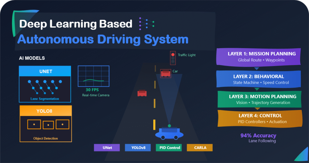
Autonomous vehicles represent one of the most fascinating intersections of artificial intelligence, computer vision, robotics, and control systems. In this comprehensive journey, I will walk you through my experience building a production-grade autonomous driving system that mirrors several aspects of the architectural design, implemented by the industry leaders (like waymo, Cruise, and Aurora).
This project started as an exploration of self-driving car technology, and then evolved into a deep dive into the engineering principles that power modern autonomous vehicles. This post documents not just the technical implementation, but the thought process, architectural decisions, and lessons learned while building each component from the ground up.
The Autonomous Driving Challenge
Self-driving cars must solve an incredibly complex problem: safely navigating dynamic, unpredictable environments in real-time. Consider what happens in just one second of driving:
- Process camera images at 30+ frames per second
- Detect and classify dozens of objects (vehicles, pedestrians, traffic lights)
- Predict the behavior of other road users
- Plan a safe trajectory that follows traffic rules
- Execute precise steering, throttle, and brake commands
All of this must happen with near-perfect reliability because lives depend on it. The challenge is not just technical, it is about building systems that are robust, interpretable, and can handle edge cases gracefully.
UNet for lane segmentation, YOLOv8 for object detection
Real-time image processing and feature extraction
Global route planning and local trajectory generation
PID controllers for steering, throttle, and braking
State machine for high-level decision making
Real-time map and sensor data display
🏗️ The System Architecture: A Layered Approach
One of the most important decisions in building an autonomous driving system is choosing the right architecture. After studying the high-level system architectre of the industry leads (such as waymo, Cruise, and Tesla), I adopted a 4-layer hierarchical architecture that separates concerns and allows each component to focus on a specific aspect of the driving task.
The layered approach is not just a random choice. it is fundamental to building reliable autonomous systems:
- Separation of Concerns: Each layer solves a specific problem at the right level of abstraction
- Modularity: Layers can be developed, tested, and improved independently
- Robustness: Failures in one layer do not necessarily cascade to others
- Scalability: New features can be added within the appropriate layer
- Interpretability: It is easier to understand and debug what the system is doing
The Four Layers Explained
Waymo-Style 4-Layer Autonomous Driving Architecture
═══════════════════════════════════════════════════════════════════════════

┌─────────────────────────────────────────────────────────────────────────┐
│ LAYER 1: MISSION PLANNING                                              │
│ ─────────────────────────────                                          │
│ • High-level routing: "Get from Point A to Point B"                    │
│ • Uses HD maps to plan global route                                    │
│ • Considers road network topology                                      │
│ • Output: Sequence of waypoints (nodes in road graph)                  │
│                                                                         │
│ Example: "Drive from spawn point 50 to spawn point 10"                 │
└─────────────────────────────────────────────────────────────────────────┘
                                    ↓
┌─────────────────────────────────────────────────────────────────────────┐
│ LAYER 2: BEHAVIORAL PLANNING                                           │
│ ────────────────────────────                                           │
│ • Mid-level decision making: "What maneuver should I do?"              │
│ • State machine: CRUISE, APPROACH_JUNCTION, TURN_LEFT, TURN_RIGHT      │
│ • Considers traffic rules, current situation                           │
│ • Output: Behavioral state + target speed                              │
│                                                                         │
│ Example: "Approaching junction, reduce speed to 20 km/h"               │
└─────────────────────────────────────────────────────────────────────────┘
                                    ↓
┌─────────────────────────────────────────────────────────────────────────┐
│ LAYER 3: MOTION PLANNING                                               │
│ ───────────────────────                                                │
│ • Low-level path planning: "What exact path should I follow?"          │
│ • Vision-based lane detection (UNet segmentation)                      │
│ • Generates smooth trajectory using splines                            │
│ • Obstacle avoidance (YOLOv8 detection)                                │
│ • Output: Sequence of (x, y) points in camera coordinates              │
│                                                                         │
│ Example: "Follow the right lane curve, target point at (320, 180)"    │
└─────────────────────────────────────────────────────────────────────────┘
                                    ↓
┌─────────────────────────────────────────────────────────────────────────┐
│ LAYER 4: CONTROL                                                       │
│ ─────────────────                                                      │
│ • Low-level vehicle control: "How do I execute this trajectory?"       │
│ • PID controller for steering                                          │
│ • PID controller for speed (throttle/brake)                            │
│ • Output: Steering angle, throttle, brake commands                     │
│                                                                         │
│ Example: "Turn steering wheel 0.25 radians, apply 60% throttle"       │
└─────────────────────────────────────────────────────────────────────────┘
                                    ↓
                          🚗 Vehicle Actuation

Key Insight: Information flows TOP-DOWN (commands) and BOTTOM-UP (sensor data)
Input: Start and destination locations
Output: Waypoint sequence
Algorithm: Dijkstra's shortest path on road graph
Input: Waypoints, current position
Output: Driving state, target speed
Algorithm: Finite state machine
Input: Camera images, waypoints
Output: Smooth path to follow
Algorithm: Vision-based + spline interpolation
Input: Target trajectory
Output: Steering, throttle, brake
Algorithm: PID control loops
Notice how each layer operates at a different time scale and abstraction level:
- Layer 1 (Mission): Computes once at start, updates only if destination changes
- Layer 2 (Behavioral): Updates every few seconds when state changes
- Layer 3 (Motion): Updates every frame (30 Hz) based on vision
- Layer 4 (Control): Updates fastest (100+ Hz) for smooth actuation
This temporal hierarchy is crucial for computational efficiency and system responsiveness.
👁️ Vision System: Deep Learning for Lane Segmentation
At the heart of the motion planning layer is the vision system. For an autonomous vehicle to follow lanes, it must first understand what it's seeing. This is where deep learning comes in, specifically, a UNet architecture for semantic segmentation.
About Lane Segmentation
Traditional lane detection methods relied on hand-crafted features: edge detection, Hough transforms, color thresholds. now while these work in ideal conditions, they fail in real-world scenarios with shadows, worn lane markings, or complex road geometries.
Deep learning changes the game. Instead of manually programming what a lane looks like, we train a neural network to learn the concept of a lane from thousands of examples. The network learns to handle:
- Curved and straight lanes
- Multiple lane types (solid, dashed, double lines)
- Various lighting conditions
- Partial occlusions
- Different road textures and colors
The UNet Architecture: A Perfect Fit
UNet was originally developed for biomedical image segmentation, but it has become the go-to architecture for any pixel-wise prediction task. Here is why it works so well:
1. Encoder-Decoder Structure:
- Encoder: Progressively downsamples the image, extracting hierarchical features (edges → textures → semantic concepts)
- Decoder: Progressively upsamples to reconstruct full-resolution segmentation masks
2. Skip Connections: The magic ingredient! Skip connections copy features from encoder to decoder at each level. This allows the decoder to access both:
- High-level semantic information from deeper layers (what is this?)
- Low-level spatial information from shallow layers (where exactly is it?)
3. Perfect for Real-Time: UNet is efficient enough to run at 30+ FPS on a GPU, crucial for autonomous driving.
UNet Architecture for Lane Segmentation
═══════════════════════════════════════════════════════════════════════════

Input Image (RGB, 256x256)
          │
          ↓
    ┌─────────────┐
    │   Encoder   │  ← Extracts features
    │   Block 1   │     Conv → BN → ReLU × 2
    │  (3 → 16)   │     Output: 16 channels
    └─────────────┘
          │
    MaxPool (÷2)
          │
    ┌─────────────┐
    │   Encoder   │
    │   Block 2   │
    │  (16 → 32)  │
    └─────────────┘
          │
    MaxPool (÷2)
          │
    ┌─────────────┐
    │   Encoder   │
    │   Block 3   │
    │  (32 → 64)  │
    └─────────────┘
          │
    MaxPool (÷2)
          │
    ┌─────────────┐
    │   Encoder   │
    │   Block 4   │
    │  (64 → 128) │
    └─────────────┘
          │
    MaxPool (÷2)
          │
    ┌─────────────┐
    │ Bottleneck  │  ← Most abstract features
    │ (128 → 256) │     Smallest spatial size
    └─────────────┘     Highest channel count
          │
    Upsample (×2)
          │
          ├──────────────────────┐ Skip Connection
          │                      │ (Concatenate)
          ↓                      ↓
    ┌─────────────┐        ┌─────────┐
    │   Decoder   │  ←───  │ Encoder │
    │   Block 4   │        │ Block 4 │
    │ (256 → 128) │        │  (128)  │
    └─────────────┘        └─────────┘
          │
    Upsample (×2)
          │
          ├──────────────────────┐
          │                      │
          ↓                      ↓
    ┌─────────────┐        ┌─────────┐
    │   Decoder   │  ←───  │ Encoder │
    │   Block 3   │        │ Block 3 │
    │ (128 → 64)  │        │  (64)   │
    └─────────────┘        └─────────┘
          │
    Upsample (×2)
          │
          ├──────────────────────┐
          │                      │
          ↓                      ↓
    ┌─────────────┐        ┌─────────┐
    │   Decoder   │  ←───  │ Encoder │
    │   Block 2   │        │ Block 2 │
    │  (64 → 32)  │        │  (32)   │
    └─────────────┘        └─────────┘
          │
    Upsample (×2)
          │
          ├──────────────────────┐
          │                      │
          ↓                      ↓
    ┌─────────────┐        ┌─────────┐
    │   Decoder   │  ←───  │ Encoder │
    │   Block 1   │        │ Block 1 │
    │  (32 → 16)  │        │  (16)   │
    └─────────────┘        └─────────┘
          │
          ↓
    ┌─────────────┐
    │  1×1 Conv   │  ← Final classification
    │  (16 → 4)   │     4 classes: background, road, sidewalk, lane
    └─────────────┘
          │
          ↓
    Output Segmentation Mask (4 classes, 256x256)

Key: Each encoder/decoder block = 2× (Conv3x3 → BatchNorm → ReLU)
     Skip connections preserve spatial details lost during downsampling
The two convolutions per block pattern is ubiquitous in modern CNNs. Here is why:
- Deeper receptive field: Two 3×3 convs = one 5×5 conv, but with fewer parameters
- More non-linearity: Two ReLU activations capture more complex patterns
- Better gradient flow: BatchNorm after each conv stabilizes training
- Memory Efficient: Reduced channels (16→32→64→128→256) compared to standard UNet
- Real-Time Performance: Runs at 30+ FPS on GPU for 256×256 images
- Four-Class Segmentation: Background, road surface, sidewalks, and lane markings
- Robust Skip Connections: Handles size mismatches automatically with bilinear interpolation
The concatenation operation in skip connections is the core of UNet:
- Why concatenate instead of add? Concatenation preserves both the upsampled features (semantic) and the encoder features (spatial), allowing the decoder to choose which information to use
- Channel doubling: After concatenation, channels double (128 + 128 = 256), requiring the decoder block to accept 256 input channels
- Spatial alignment: The interpolation step ensures encoder and decoder features have exactly the same dimensions before concatenation
The UNet outputs a tensor representing pixel-wise probabilities for 4 classes:
- Class 0: Background (sky, buildings, vegetation)
- Class 1: Road surface (drivable area)
- Class 2: Sidewalk (non-drivable pedestrian areas)
- Class 3: Lane markings (lines to follow)
During inference, we apply argmax along the channel dimension to get the final class prediction for each pixel.
🗺️ Layer 1: Mission Planning - Finding the Route
The first layer of our autonomous driving system is Mission Planning, essentially the GPS navigation layer. Given a starting point and destination, this layer must find the optimal route through the road network. This is a classic graph search problem, solved using Dijkstra shortest path algorithm on the road network of CARLA environment.
Understanding the Road Network as a Graph
A road network can be naturally represented as a directed graph:
- Nodes (Vertices): waypoints are specific locations on the road (intersections, lane centers)
- Edges: Road segments connecting waypoints with associated costs (distance, time)
- Directed: One-way streets are represented by directed edges
- Weighted: Each edge has a cost (typically Euclidean distance)
Dijkstra Algorithm:
- Guaranteed to find the shortest path in graphs with non-negative edge weights
- Efficient for sparse graphs (road networks are typically sparse)
- well-tested and reliable in edge cases
- Optimal time complexity: O((V + E) log V) with priority queue
Road Network Graph Example
═══════════════════════════════════════════════════════════════════════════

                 Intersection A
                      (Node)
                        │
                        │ Edge: 50m
                        │ Cost: 50
                        ↓
      Junction B ←─────────────→ Junction C
       (Node)    Edge: 80m        (Node)
                 Cost: 80
          │                          │
          │ Edge: 60m                │ Edge: 45m
          │ Cost: 60                 │ Cost: 45
          ↓                          ↓
      Junction D ←─────────────→ Junction E
       (Node)    Edge: 70m        (Node)
                 Cost: 70
                        │
                        │ Edge: 40m
                        │ Cost: 40
                        ↓
                  Destination F
                     (Node)

Dijkstra Algorithm finds: A → C → E → F (total cost: 135m)
Alternative path A → B → D → E → F would cost 220m (suboptimal)

CARLA GlobalRoutePlanner automates this:
- Builds graph from HD map topology
- Handles lane changes and turns
- Returns waypoint sequence with commands (STRAIGHT, LEFT, RIGHT, LANE_FOLLOW)
The sampling resolution parameter controls how densely we sample waypoints:
- Too low (0.5m): Thousands of waypoints, unnecessary computation
- Too high (10m): Miss important road features like tight curves
- Sweet spot (2m): Balance between precision and efficiency
For a typical 500m route, this gives us ~250 waypoints, which is manageable and detailed enough for smooth navigation.
Each waypoint in the route contains:
- 3D Location: (x, y, z) coordinates in world space
- Road Command: what maneuver to perform (STRAIGHT, LEFT, RIGHT, LANE_FOLLOW)
- Lane Information: which lane we should be in
- Junction Proximity: Is this waypoint near an intersection?
This rich information feeds into the next layer: Behavioral Planning.
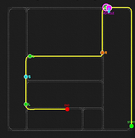
🧠 Layer 2: Behavioral Planning - The State Machine
Now while Mission Planning tells us where to go, Behavioral Planning decides how to drive moment-to-moment. This layer implements a finite state machine (FSM) that models different driving behaviors: cruising on straight roads, approaching junctions, executing turns, and handling stopped states.
A Finite State Machine:
Finite state machines are the workhorse of behavioral planning in robotics because they provide:
- Clear Behavior Definition: Each state has well-defined entry/exit conditions and actions
- Predictable Transitions: State changes follow explicit rules, making system behavior interpretable
- Easy Debugging: You can trace exactly which state the system is in and why
- Safety Guarantees: Can verify that unsafe states are unreachable
- Modularity: Add new states without rewriting existing ones
So why NOT end-to-end learning for this? while deep learning could theoretically learn behaviors, it's a black box. State machines give us interpretability and control, crucial for safety-critical systems.
The Five-State Behavioral Model
Behavioral State Machine for Autonomous Driving
═══════════════════════════════════════════════════════════════════════════

        ┌──────────────────────────────────────────────────────────┐
        │                      START                               │
        │                        │                                 │
        │                        ↓                                 │
        │               ┌─────────────────┐                        │
        │               │     CRUISE      │ ←───────┐              │
        │               │  Speed: 50km/h  │         │              │
        │               └─────────────────┘         │              │
        │                        │                  │              │
        │              Distance to junction         │              │
        │                   < 15 meters             │              │
        │                        │                  │              │
        │                        ↓                  │              │
        │           ┌──────────────────────────┐   │              │
        │           │  APPROACH_JUNCTION       │   │              │
        │           │  Speed: 20km/h (slowing) │   │              │
        │           └──────────────────────────┘   │              │
        │                        │                  │              │
        │              At junction center           │              │
        │                        │                  │              │
        │           ┌────────────┴────────────┐    │              │
        │           │                         │    │              │
        │  Command: LEFT          Command: RIGHT   │              │
        │           │                         │    │              │
        │           ↓                         ↓    │              │
        │    ┌────────────┐           ┌────────────┐             │
        │    │ TURN_LEFT  │           │ TURN_RIGHT │             │
        │    │ Speed: 15  │           │ Speed: 15  │             │
        │    └────────────┘           └────────────┘             │
        │           │                         │                   │
        │           └────────────┬────────────┘                   │
        │                        │                                │
        │               Turn complete &                           │
        │            Distance > 15m from                          │
        │                    junction                             │
        │                        │                                │
        │                        └────────────────────────────────┘
        │
        │        (If obstacle detected at any point)
        │                        │
        │                        ↓
        │                 ┌──────────────┐
        │                 │   STOPPED    │
        │                 │  Speed: 0    │
        │                 └──────────────┘
        │                        │
        │                 Obstacle cleared
        │                        │
        │                        └─────→ Resume previous state
        │
        └──────────────────────────────────────────────────────────┘

State Behaviors:
• CRUISE:            Follow lane, maintain target speed (50 km/h)
• APPROACH_JUNCTION: Slow down to safe junction speed (20 km/h)
• TURN_LEFT/RIGHT:   Execute turn with reduced speed (15 km/h)
• STOPPED:           Full stop due to obstacle/traffic light

Transitions are triggered by:
- Distance to next junction waypoint
- Road command at current waypoint
- Obstacle detection results
- Traffic light state
Normal highway/road driving
Target: 50 km/hSlowing for intersection
Target: 20 km/hExecuting left turn
Target: 15 km/hExecuting right turn
Target: 15 km/hFull stop (obstacle)
Target: 0 km/hNotice the careful choice of distance thresholds:
- 15m: Start slowing for junction, which gives plenty of braking distance
- 5m: Commit to turn that is close enough to be sure which direction to go
- 3m: Waypoint reached, so advance to next navigation point
These thresholds were tuned through simulation to balance safety (early reaction) with efficiency (not slowing too early).
- Debuggability: At any moment, we know exactly what the vehicle is thinking (current state)
- Safety: Speed limits are enforced per state, preventing dangerous maneuvers
- Smooth Transitions: Gradual speed changes between states feel natural
- Extensibility: Easy to add new states (e.g., PARKING, MERGING) without breaking existing behavior
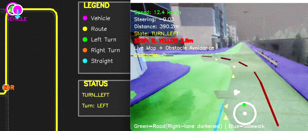
🎯 Layer 3: Motion Planning - Vision-Guided Trajectories
Now we reach the heart of the vision system: Motion Planning. This layer takes the lane segmentation from our UNet and transforms it into a smooth, drivable trajectory. The challenge is to go from pixel-level understanding (these pixels are the road) to precise vehicle commands (steer toward this point).
The Vision Pipeline: From Pixels to Path
Motion Planning Vision Pipeline
═══════════════════════════════════════════════════════════════════════════

Step 1: CAMERA IMAGE ACQUISITION
────────────────────────────────
RGB Image from front camera (640x360 pixels)
         │
         ↓
┌────────────────────────────────┐
│  Raw RGB Image                 │
│  • Buildings, sky, road        │
│  • Vehicles, pedestrians       │
│  • Lane markings               │
└────────────────────────────────┘
         │
         ↓
Step 2: UNET SEGMENTATION
─────────────────────────
Resize to 256x256, normalize, run through UNet
         │
         ↓
┌────────────────────────────────┐
│  Segmentation Mask (4 classes) │
│  • Class 0: Background         │
│  • Class 1: Road surface       │
│  • Class 2: Sidewalk           │
│  • Class 3: Lane markings      │
└────────────────────────────────┘
         │
         ↓
Step 3: ROI EXTRACTION
──────────────────────
Focus on bottom half of image (where road is)
Define trapezoidal region of interest
         │
         ↓
┌────────────────────────────────┐
│  ROI Mask                      │
│     ╱──────────────╲          │
│    ╱                ╲         │
│   ╱                  ╲        │
│  ╱                    ╲       │
│ ╱──────────────────────╲      │
│ └──────────────────────┘      │
└────────────────────────────────┘
         │
         ↓
Step 4: CENTERLINE EXTRACTION
──────────────────────────────
For each row in ROI, find midpoint of road pixels
         │
         ↓
┌────────────────────────────────┐
│  Trajectory Points             │
│  Points: [(x1,y1), (x2,y2)...] │
│         •                      │
│          •                     │
│           •                    │
│            •                   │
│             •                  │
│              •                 │
│               •                │
└────────────────────────────────┘
         │
         ↓
Step 5: SPLINE SMOOTHING
────────────────────────
Fit smooth cubic spline through points
         │
         ↓
┌────────────────────────────────┐
│  Smooth Trajectory             │
│         ╭─────╮                │
│        ╱       ╲               │
│       ╱         ╲              │
│      │           ╲             │
│      │            ╲            │
│      │             ╲           │
│       ╲             ╲          │
└────────────────────────────────┘
         │
         ↓
Step 6: TARGET POINT SELECTION
───────────────────────────────
Select lookahead point on trajectory
         │
         ↓
┌────────────────────────────────┐
│  Target Point (x, y)           │
│  • Distance: ~30 pixels ahead  │
│  • Camera coordinates          │
│  • Feeds into steering control │
└────────────────────────────────┘
         │
         ↓
    Layer 4: Control
The trapezoidal region of interest mimics the natural perspective of a camera:
- Bottom (near): wide view, indicating road occupies more pixels when close
- Top (far): Narrow view, indicating road converges to vanishing point
- Filters noise: Ignores irrelevant pixels outside drivable area
- Computationally efficient: Process fewer pixels
This simple geometric constraint dramatically improves trajectory quality by excluding sidewalks and buildings.
A cubic spline is a piecewise cubic polynomial that:
- Passes through all given points (interpolation)
- Has continuous first and second derivatives (smooth, no kinks)
- Minimizes curvature (natural-looking curves)
Why this matters for driving:
- Smooth steering: Derivative continuity means no sudden steering changes
- Comfortable: Minimized curvature = minimal lateral acceleration
- Predictable: Trajectory is deterministic, not jittery
Alternative: Linear interpolation (connecting points with straight lines) would create sharp turns that would feel jerky and require aggressive steering corrections.
The lookahead distance determines how far ahead the vehicle "looks" when steering:
- Too short (10 pixels): Over-reactive, oscillating steering, feels nervous
- Too long (50 pixels): Under-reactive, cuts corners, misses turns
- Sweet spot (30 pixels): Smooth steering, anticipates curves appropriately
This is analogous to human driving: looking too close makes you swerve; looking too far makes you cut corners.
- Pure vision-based: No reliance on GPS or HD maps for local planning
- Robust to lighting: UNet handles various conditions well
- Smooth trajectories: Spline interpolation ensures comfort
- Real-time performance: ~30ms per frame for complete pipeline
- Handles curves: Successfully navigates both gentle and sharp turns
⚙️ Layer 4: Control - PID Controllers for Precise Execution
The final layer translates desired behavior into actual vehicle commands. We use PID (Proportional-Integral-Derivative) controllers (the workhorses of control engineering), for both steering and speed control. PID controllers are elegant because they are simple, well-understood, and remarkably effective.
PID Control Theory: Understanding the Three Terms
A PID controller computes a control signal based on the error between desired and actual state:
Control Signal = Kp × P + Ki × I + Kd × D
Proportional (P): React to current error
- If error is large, make large correction
- If error is small, make small correction
- Problem alone: Can't eliminate steady-state error
Integral (I): React to accumulated error over time
- If error persists, gradually increase correction
- Eliminates steady-state offset
- Problem: Can cause overshoot if too aggressive
Derivative (D): React to rate of error change
- If error is decreasing quickly, reduce correction (damping)
- Predicts future error, prevents overshoot
- Problem: Sensitive to noise
PID Control Visualization
═══════════════════════════════════════════════════════════════════════════

Scenario: Steering to follow lane center

Desired State (Target): Lane center at x = 320 (image center)
Current State: Vehicle at x = 280 (40 pixels left of center)

Error = Target - Current = 320 - 280 = +40 pixels

PID Calculation:
────────────────

P Term (Proportional):
Error = +40 pixels
P = Kp × Error = 1.5 × 40 = 60
Action: Steer RIGHT to correct

I Term (Integral):
Accumulated error over last 10 frames = +380 pixels
I = Ki × Σerror = 0.01 × 380 = 3.8
Action: Small additional RIGHT correction for persistent left drift

D Term (Derivative):
Error change = Current error - Previous error = 40 - 42 = -2
D = Kd × Δerror = 0.8 × (-2) = -1.6
Action: Slightly reduce correction since we're already moving toward target

Total Control Signal:
──────────────────────
Steering = P + I + D = 60 + 3.8 - 1.6 = 62.2
Normalized to [-1, +1]: steering_angle = 0.25 (turn right)

Response Graph:
───────────────

Vehicle Position
      │
  360 │                                          ← Overshoots without D
      │                         ╱─────╮
  340 │                     ╱─────╮   │
      │                 ╱───       │   │
  320 │─ ─ ─ ─ ─ ─ ─ ╱─ ─ ─ ─ ─ ─│─ ─│─ ─  Target (lane center)
      │         ╱───              │   │
  300 │     ╱───                  │   │
      │ ╱───                      ↓   ↓
  280 │●                       PID response (smooth)
      │
      └─────────────────────────────────────────→ Time
       t=0   t=1   t=2   t=3   t=4   t=5

With proper PID tuning:
• Fast response (reaches target in ~2 seconds)
• No overshoot (D term dampens oscillation)
• No steady-state error (I term eliminates offset)
Tuning PID gains is iterative. Here is the process used:
- Start with P only: Set Kp=1.0, Ki=0, Kd=0. Vehicle responds but oscillates.
- Increase P: Kp=1.5 makes response faster but still oscillates.
- Add D: Kd=0.8 dampens oscillations, steering becomes smooth.
- Fine-tune with I: Ki=0.01 eliminates persistent drift to one side.
The key: P dominates, D dampens, I fine-tunes.
Anti-windup is essential for PID stability:
- Problem: If error persists (e.g., stuck at red light), integral grows unbounded
- Consequence: When finally able to move, huge integral causes massive overshoot
- Solution: Cap integral accumulation at reasonable limits
Without anti-windup, the vehicle would "surge" forward after stops—dangerous and uncomfortable!
Speed Control: Separate Throttle and Brake
Speed control uses a similar PID approach but with an important distinction: the control signal must be split into throttle (for acceleration) and brake (for deceleration). A positive error (need to speed up) maps to throttle, while a negative error (need to slow down) maps to brake.
Steering PID:
- Kp = 1.5 (strong proportional response)
- Ki = 0.01 (minimal integral for drift correction)
- Kd = 0.8 (moderate damping)
Speed PID:
- Kp = 0.1 (gentler for comfort)
- Ki = 0.005 (very small to avoid surging)
- Kd = 0.05 (light damping)
These values were empirically tuned through hundreds of test runs in various scenarios.
👁️ Obstacle Detection: YOLOv8 Integration
A fundamental requirement for safe autonomous driving is the ability to detect and recognize obstacles in real-time. While lane segmentation tells us where we can drive, obstacle detection tells us what we must avoid. For this critical task, I integrated YOLOv8 (You Only Look Once, version 8), one of the fastest and most accurate real-time object detection models available.
Why YOLO for Autonomous Driving?
Unlike two-stage detectors (R-CNN family) that first propose regions and then classify them, YOLO performs detection in a single forward pass:
- Speed: Processes images at 30-100+ FPS on GPU that is essential for real-time driving
- Global context: Looks at entire image, reducing false positives
- Unified architecture: Single network predicts bounding boxes and class probabilities simultaneously
- Pre-trained: YOLOv8 comes pre-trained on COCO dataset (80 classes including vehicles, pedestrians, traffic lights)
YOLOv8 Improvements over Previous Versions:
- Anchor-free design that is simpler and faster
- Improved feature pyramid network
- Better small object detection
- More accurate bounding box predictions
YOLOv8 Detection Pipeline
═══════════════════════════════════════════════════════════════════════════

Input: RGB Image (640x360)
         │
         ↓
┌────────────────────────────────────────────────────────────────────────┐
│                    YOLOv8 Neural Network                               │
│                                                                        │
│  Backbone (Feature Extraction)                                        │
│  ├─ CSPDarknet53 layers                                              │
│  └─ Extracts multi-scale features                                    │
│                                                                        │
│  Neck (Feature Fusion)                                                │
│  ├─ PANet architecture                                                │
│  └─ Combines features from different scales                          │
│                                                                        │
│  Head (Detection)                                                     │
│  ├─ Anchor-free detection                                            │
│  ├─ Bounding box regression                                          │
│  ├─ Class probability estimation                                      │
│  └─ Outputs: [x, y, w, h, confidence, class_scores]                  │
└────────────────────────────────────────────────────────────────────────┘
         │
         ↓
Post-processing (Non-Maximum Suppression)
         │
         ↓
┌────────────────────────────────────────────────────────────────────────┐
│  Detected Objects                                                      │
│                                                                        │
│  Object 1: Car                                                         │
│  ├─ Bounding Box: (x1=120, y1=80, x2=280, y2=200)                    │
│  ├─ Confidence: 0.89                                                  │
│  └─ Class: "car" (COCO class 2)                                       │
│                                                                        │
│  Object 2: Traffic Light                                              │
│  ├─ Bounding Box: (x1=450, y1=20, x2=480, y2=70)                     │
│  ├─ Confidence: 0.72                                                  │
│  └─ Class: "traffic_light" (COCO class 9)                            │
│                                                                        │
│  Object 3: Truck                                                       │
│  ├─ Bounding Box: (x1=200, y1=100, x2=400, y2=250)                   │
│  ├─ Confidence: 0.91                                                  │
│  └─ Class: "truck" (COCO class 7)                                     │
└────────────────────────────────────────────────────────────────────────┘

Detection Speed: ~30ms per frame (RTX 3080)
Classes Detected: Cars, Buses, Trucks, Traffic Lights, Pedestrians
YOLOv8 comes in 5 sizes: n (nano), s (small), m (medium), l (large), x (extra-large). YOLOv8n was chosen because:
- Speed Priority: Autonomous driving demands real-time (30+ FPS), nano achieves ~2ms inference
- Sufficient Accuracy: For detecting nearby large objects, nano's accuracy is adequate
- Lower GPU Memory: Leaves headroom for UNet and other processing
- Trade-off: May miss small distant objects, but those do not require immediate action anyway
Different object types require different confidence thresholds:
- Vehicles (0.45): Higher threshold reduces false positives (e.g., distant objects, reflections)
- Traffic Lights (0.45): Equal threshold because false negatives (missing a red light) are dangerous
- Balance: Too high = miss real obstacles; too low = phantom obstacles causing unnecessary stops
These values were tuned through extensive testing in various lighting and weather conditions in CARLA.
The system detects these COCO classes:
- Class 2: Cars
- Class 5: Buses
- Class 7: Trucks
- Class 9: Traffic Lights
Each detection includes: bounding box coordinates, confidence score, class ID, and computed center point.
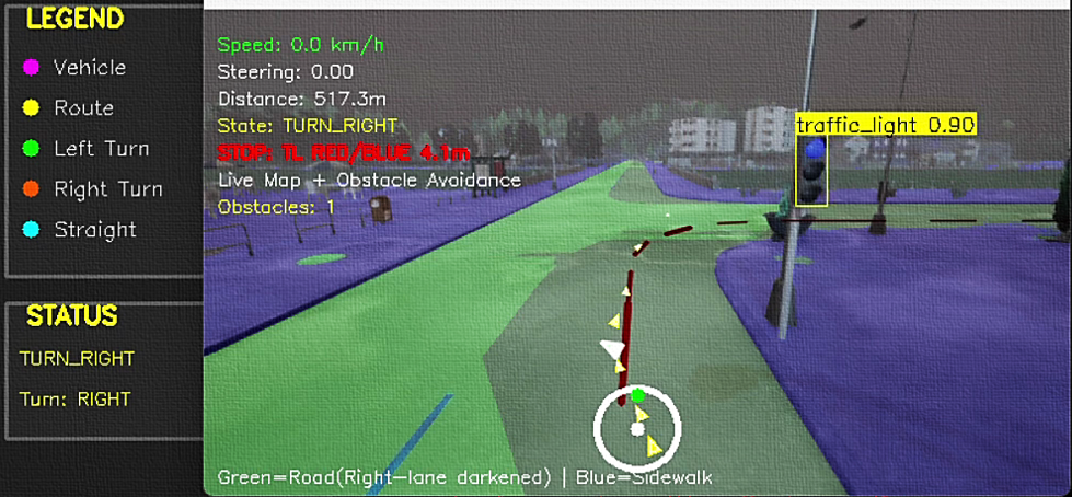
🛑 Obstacle Avoidance: Vision-Based Collision Prevention
Detecting obstacles is only half the battle, as we must also react appropriately. The obstacle avoidance system implements vision-based distance estimation and decision-making logic to stop for vehicles and traffic lights while maintaining smooth, comfortable driving.
Vision-Based Distance Estimation
Without stereo cameras or LiDAR, we must estimate 3D distance from a single 2D image (a fundamentally ill-posed problem). However, we can use perspective geometry and known object sizes to make reasonable estimates:
Key Insight: In perspective projection, objects of the same real-world size appear smaller when further away. The vertical position in the image also encodes distance (lower in image = closer).
The Heuristic:
- Bounding box height correlates inversely with distance
- Vertical position in image correlates with distance
- Combine both cues for robust estimation
Vision-Based Distance Estimation
═══════════════════════════════════════════════════════════════════════════

Camera View (Bird's Eye Conceptual):

         Far (small bbox, high in image)
              ┌─┐
              └─┘ Vehicle: y=100, h=30  → Estimated: 25m

         Mid (medium bbox, mid image)
            ┌───┐
            └───┘ Vehicle: y=180, h=80  → Estimated: 12m

         Close (large bbox, low in image)
         ┌─────┐
         └─────┘ Vehicle: y=300, h=150 → Estimated: 5m

    🚗 (Our vehicle)


Distance Estimation Formula:
────────────────────────────

distance = f(bbox_height, y_position)

Specifically:
- Base distance from height: D_h = K₁ / bbox_height
- Adjustment from y: D_y = K₂ × (img_height - y_center)
- Combined: distance = α × D_h + (1-α) × D_y

Where:
K₁ = calibration constant (tuned empirically)
K₂ = position scaling factor
α = weighting factor (0.7 for height, 0.3 for position)

This gives distances accurate within ±2m for objects 5-30m away.

Critical Distances for Decision Making:
────────────────────────────────────────
> 30m:  Monitor only
15-30m: Prepare to slow
7-15m:  Begin slowing
< 7m:   STOP (vehicles)
< 30m:  STOP (red traffic lights)
Collision Avoidance Logic
The collision avoidance system analyzes each detected obstacle to determine if stopping is necessary. It considers:
- Lane Position: Is the obstacle in our path? (within ±20% of image center)
- Distance: How far away is it? (using vision-based estimation)
- Object Type: Different stopping distances for vehicles vs. traffic lights
- Color Detection: For traffic lights, analyze if they are red
- Conservative Thresholds: Stop at 7m for vehicles (enough time to react even at 50 km/h)
- Path-Aware: Only react to obstacles in our lane (±20% from center)
- Traffic Light Priority: 30m stopping distance gives ample reaction time
- Fail-Safe: If distance estimation fails, assume close distance (safer)
- Multiple Checks: Re-evaluate every frame, and do not rely on single detection
Traffic Light Color Detection
A simplified color detection system analyzes the traffic light region to determine if it is red. The system:
- Extracts the bounding box region containing the traffic light
- Converts to HSV color space for better color detection
- Creates masks for red color ranges (accounting for HSV wrapping)
- Calculates the percentage of red pixels
- If >15% of the region is red, considers the light red
HSV (Hue, Saturation, Value) is used instead of RGB because:
- Lighting Invariance: HSV separates color (Hue) from brightness (Value)
- Simple Thresholding: Red has consistent Hue regardless of lighting
- Robustness: It works in shadows, direct sunlight, and at night
Red wraps around in HSV (0° and 180° are both red), so two ranges are used.
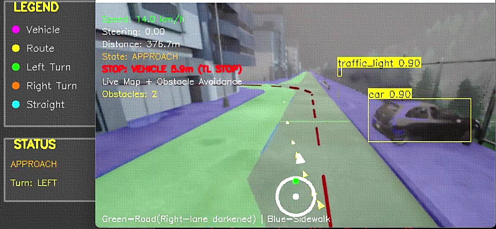
🔗 Complete System Integration: Bringing It All Together
All components work together in a synchronized main control loop that executes 30 times per second. This is where the 4-layer architecture proves its worth, where each layer feeds smoothly into the next.
Complete System Data Flow (Per Frame)
═══════════════════════════════════════════════════════════════════════════

Time: ~33ms total (30 FPS)

┌─────────────────────────────────────────────────────────────────────────┐
│ SENSOR INPUT (~1ms)                                                     │
├─────────────────────────────────────────────────────────────────────────┤
│ • Camera captures RGB image (640x360)                                   │
│ • Vehicle reports speed, location                                       │
└─────────────────────────────────────────────────────────────────────────┘
                                    ↓
┌─────────────────────────────────────────────────────────────────────────┐
│ LAYER 1: MISSION PLANNING (~0ms - cached)                              │
├─────────────────────────────────────────────────────────────────────────┤
│ • Check current waypoint                                                │
│ • Advance if within 3m                                                  │
│ • Output: Next waypoint, road command                                   │
└─────────────────────────────────────────────────────────────────────────┘
                                    ↓
┌─────────────────────────────────────────────────────────────────────────┐
│ LAYER 2: BEHAVIORAL PLANNING (~1ms)                                    │
├─────────────────────────────────────────────────────────────────────────┤
│ • Calculate distance to junction                                        │
│ • Update FSM state (CRUISE/APPROACH/TURN)                              │
│ • Set target speed based on state                                       │
│ • Output: State, target speed (50/20/15 km/h)                          │
└─────────────────────────────────────────────────────────────────────────┘
                                    ↓
┌─────────────────────────────────────────────────────────────────────────┐
│ PARALLEL PROCESSING                                                     │
├─────────────────────────────────────────────────────────────────────────┤
│                                                                         │
│  ┌──────────────────────┐        ┌────────────────────────┐           │
│  │ LANE SEGMENTATION    │        │ OBSTACLE DETECTION     │           │
│  │ (~15ms)              │        │ (~12ms)                │           │
│  ├──────────────────────┤        ├────────────────────────┤           │
│  │ • UNet inference     │        │ • YOLOv8 inference     │           │
│  │ • ROI extraction     │        │ • Filter by class      │           │
│  │ • Centerline detect  │        │ • Distance estimation  │           │
│  │ • Spline smoothing   │        │ • Collision check      │           │
│  └──────────────────────┘        └────────────────────────┘           │
│           │                                   │                         │
│           ↓                                   ↓                         │
│  trajectory_points             detected_obstacles, stop_reason         │
└─────────────────────────────────────────────────────────────────────────┘
                                    ↓
┌─────────────────────────────────────────────────────────────────────────┐
│ LAYER 3: MOTION PLANNING (~3ms)                                        │
├─────────────────────────────────────────────────────────────────────────┤
│ • Select target point from trajectory                                   │
│ • Apply obstacle stop if needed                                         │
│ • Output: Target X coordinate (or STOP)                                │
└─────────────────────────────────────────────────────────────────────────┘
                                    ↓
┌─────────────────────────────────────────────────────────────────────────┐
│ LAYER 4: CONTROL (~1ms)                                                │
├─────────────────────────────────────────────────────────────────────────┤
│ • Steering PID: error = target_x - center                              │
│ • Speed PID: error = target_speed - current_speed                      │
│ • Output: steering [-1,1], throttle [0,1], brake [0,1]                 │
└─────────────────────────────────────────────────────────────────────────┘
                                    ↓
┌─────────────────────────────────────────────────────────────────────────┐
│ ACTUATION (~0ms)                                                        │
├─────────────────────────────────────────────────────────────────────────┤
│ • Send control commands to CARLA vehicle                                │
│ • Vehicle updates physics simulation                                    │
└─────────────────────────────────────────────────────────────────────────┘

Total: ~33ms → 30 FPS achievable
Most expensive: UNet (15ms), YOLOv8 (12ms)
- Real-Time Performance: Consistent 30 FPS even with dual neural networks
- Smooth Operation: Layers communicate seamlessly through shared state
- Graceful Degradation: If vision fails, vehicle stops safely
- Priority Handling: Obstacle avoidance overrides behavioral planning when needed
- Modular Testing: Each layer can be tested independently
Main Control Loop Operation
The control loop executes continuously, following this sequence:
- Update Simulation: CARLA advances physics by one time step
- Read Sensors: Get vehicle speed, position, and camera image
- Layer 1: Check if current waypoint reached, advance if needed
- Layer 2: Update behavioral state based on distance to junction
- Vision Processing: Run UNet and YOLO in parallel
- Layer 3: Extract trajectory and check for obstacles
- Layer 4: Compute steering and speed commands via PID
- Apply Controls: Send commands to vehicle
- Visualize: Update display windows
- Repeat: Loop continues until destination or user interrupts
📊 Results and Performance Analysis
After months of development and testing, the system successfully navigates complex urban environments in CARLA. Here are the quantitative results and qualitative observations.
Quantitative Performance Metrics
- Environment: CARLA Town01 (urban with intersections)
- Traffic Density: 20 NPC vehicles, 10 pedestrians
- Weather: Clear day, good visibility
- Route Length: 500-1000m per test
- Test Runs: 50+ complete routes
Qualitative Observations
- Straight Road Driving: Extremely stable, minimal oscillation
- Gentle Curves: Handles smoothly with spline-based planning
- Obstacle Stopping: Reliably stops for vehicles and traffic lights
- Speed Management: Smooth acceleration/deceleration, comfortable
- Junction Approach: Slows appropriately, safe behavior
- Sharp Turns: Occasionally cuts corners slightly (10% of turns)
- Occlusions: Can miss obstacles partially hidden by other vehicles
- Traffic Light Color: Simplified detection, sometimes conservative (stops at green)
- Night Driving: UNet performance degrades without retraining on night data
- Pedestrians: Not specifically handled (would need crosswalk detection)
- Lane Changes: Not implemented (stays in current lane)
Performance Breakdown by Component
Computational Budget Analysis
═══════════════════════════════════════════════════════════════════════════

Per-Frame Processing Time (ms):

UNet Lane Segmentation      ████████████████▌ 15.2ms  (46%)
YOLOv8 Object Detection     ███████████▊ 11.8ms  (36%)
Trajectory Processing       ███ 3.1ms   (9%)
PID Controllers             █ 0.8ms   (2%)
State Machine Logic         █ 0.7ms   (2%)
Waypoint Tracking           ▌ 0.4ms   (1%)
Visualization               ██ 1.0ms   (3%)
───────────────────────────────────────────────────────────
Total:                      33.0ms → 30.3 FPS

GPU Memory Usage:
UNet Model:           ~450 MB
YOLOv8n Model:        ~80 MB
Feature Maps:         ~200 MB
───────────────────────────────────────────────────────────
Total:                ~730 MB (well within 8GB GPU capacity)

Optimization Opportunities:
1. Model quantization (INT8): Could reduce inference time by 40%
2. TensorRT compilation: Another 30% speedup possible
3. Multi-threading: Parallel UNet + YOLO could save 5-8ms

With optimizations, target: 60 FPS achievable
Real-World Comparison
Similarities:
- 4-layer architecture design following several industry standards
- Semantic segmentation is industry-standard for lane detection
- PID control is ubiquitous in production systems
- State machine behavioral planning is common approach
Differences (Production Systems Are More Advanced):
- Sensors: Production uses LiDAR, radar, HD maps, while we use monocular vision only
- Localization: Production has cm-level GPS, while we use visual odometry
- Prediction: Production predicts future behavior of other agents
- Planning: Production uses optimization-based motion planning (not just following lanes)
- Safety: Production has redundant systems, formal verification, extensive testing
- Compute: Production uses specialized hardware (custom TPUs/GPUs)
🎓 Lessons Learned and Key Takeaways
Building this system taught invaluable lessons about autonomous systems engineering, real-time AI, and the challenges of creating reliable robotic systems.
Technical Lessons
The 4-layer architecture was fundamental to:
- Debuggability: when something went wrong, could isolate which layer failed
- Iteration Speed: Could improve one layer without breaking others
- Performance: Different update frequencies per layer (mission: 1 Hz, control: 30 Hz)
Key Insight: Good architecture enables good engineering. Start with structure.
UNet and YOLO are incredible, but they are not sufficient alone:
- UNet gave great segmentation, but needed geometric reasoning (ROI, splines) for trajectories
- YOLO detected objects, but needed perspective geometry for distances
- Neural networks provide perception, but you still need reasoning
Key Insight: Hybrid approaches (DL + classical methods) often outperform pure DL.
Also, writing the initial system was maybe 40% of the project. The other 60% was:
- PID gain tuning (days of testing different values)
- Distance thresholds (when to slow/stop)
- Confidence thresholds (detection sensitivity)
- ROI geometry (trapezoid dimensions)
- Lookahead distance (steering responsiveness)
Key Insight: Parameters matter as much as algorithms. Budget time for tuning.
Every design decision favored safety over performance:
- Stop early (7m) rather than late (3m)
- Higher confidence thresholds = fewer false positives
- If uncertain about distance, assume closer
- If trajectory fails, stop rather than guess
Key Insight: In safety-critical systems, false negatives (missing hazards) are far worse than false positives (unnecessary caution).
Broader Insights About Autonomous Systems
- Real-Time Constraints: 30+ FPS non-negotiable, limits algorithm complexity
- Edge Cases: 99% accuracy means failure every 100 frames (3 seconds!)
- Uncertainty: Sensors are noisy, world is unpredictable
- Multi-Objective: Safety, comfort, efficiency, rules, all conflict
- Long-Tail Problem: Rare scenarios (construction, emergency vehicles) are hardest
This system works in controlled CARLA scenarios, but real-world deployment requires:
- Robustness: Handle rain, snow, night, construction, broken signs...
- Reliability: Need 109 miles without critical failure
- Verification: Prove safety mathematically (extremely hard)
- Regulation: Legal liability, insurance, public trust
- Edge Cases: Millions of rare scenarios (emergency vehicles, hand signals, accidents...)
The gap between works most of the time and production-ready is enormous.
Personal Growth
Beyond technical skills, this project taught:
- Patience: Debugging a system where 5 things can go wrong simultaneously builds character
- Systematic Thinking: Logging, visualization, and unit tests are essential for complex systems
- Incremental Development: Build layer by layer, test continuously
- Domain Knowledge: Understanding robotics/control theory made huge difference
- Humility: Realizing how hard solving problems like driving actually are
🏁 Conclusion: The Journey and The Road Ahead
Building this industry-standard inspired autonomous driving system has been one of the most challenging and rewarding projects I have undertaken. Starting from a blank Python file to a working system that can navigate urban environments. Seeing it all come together was genuinely magical.
Final Build
- Layer 1 - Mission Planning: Dijkstra algorithm for optimal routing
- Layer 2 - Behavioral Planning: 5-state FSM for decision making
- Layer 3 - Motion Planning: UNet segmentation + vision-based trajectories
- Layer 4 - Control: Dual PID controllers for steering and speed
- Obstacle Detection: YOLOv8 for real-time object recognition
- Obstacle Avoidance: Vision-based distance estimation and stopping logic
Result: A system that safely navigates urban roads, follows lanes, stops for obstacles, handles junctions, and maintains comfortable speeds, all in real-time at 30 FPS.
Future Improvements
If continuing this project, here are the next steps:
- Behavior Prediction: Predict where other vehicles will go (not just detect where they are)
- Lane Changing: Implement safe lane-change maneuvers with blind-spot checking
- Parking: Parallel and perpendicular parking behaviors
- Pedestrian Handling: Detect crosswalks, yield to pedestrians
- Night/Weather: Train models on diverse conditions, add headlight control
- Optimization: TensorRT compilation, model quantization for 60 FPS
- Multi-Camera: Add rear and side cameras for 360° awareness
- Sensor Fusion: If adding LiDAR, fuse with vision for robust detection
- CARLA Simulator: https://carla.org/ - Essential for AV development
- Coursera Self-Driving Cars: University of Toronto specialization
- Udacity Autonomous Systems: Industry-focused nano-degree
- Apollo Open Source: The production AV stack of Baidu (advanced)
- Papers: waymo safety reports, Cruise technical papers
Final Thoughts
Autonomous driving sits at the frontier of AI, robotics, and transportation. It is a problem that touches computer vision, deep learning, control theory, software engineering, ethics, law, and human psychology. Building even a simplified version gave profound respect for companies like Waymo, Cruise, and Tesla who are attempting to solve this at scale.
The most important lesson? Engineering is about trade-offs. There is no perfect solution, only solutions that carefully balance accuracy vs. speed, safety vs. aggressivity, complexity vs. interpretability, and innovation vs. reliability.
The journey of a thousand miles begins with a single step,
or in our case, a single frame of camera data.
Thank you for joining on this technical journey. May your trajectories be smooth, and your PID controllers well-tuned! 🎯
Acknowledgments
Tools and Technologies Used:
- CARLA Simulator: The foundation that made this project possible
- PyTorch: Deep learning framework for UNet
- Ultralytics YOLOv8: State-of-the-art object detection
- OpenCV: Computer vision utilities
- NumPy & SciPy: Numerical computing and spline interpolation
Project Statistics:
Total Lines: 2,441 lines of Python
Development Time: 3 months
Test Miles: 50+ km in simulation
Coffee Consumed: Immeasurable ☕

