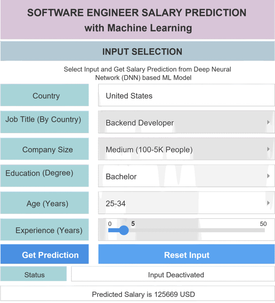
Exploring how machine learning can estimate tech salaries across countries and roles combining structured data, neural networks, and a bit of curiosity.
Building ML Model to predict Salary
An Neural Network that predicts software engineer annual salaries. Built with real-world survey data from 60,000+ professionals across 46 countries and 22 job titles.
Table of Contents
Toggle📋 Project Overview
This project addresses one of the most critical questions in tech careers: What should my salary be?
Software engineer salaries vary dramatically based on multiple factors including location, company size, experience, education, and job specialization. This project leverages machine learning to provide data-driven salary predictions by analyzing these complex relationships using survey data from real software engineers worldwide.
Key Features of the App
- ⭐ Intelligent Salary Prediction: Deep neural network model trained on 60,000+ real salary data points
- ⭐ Interactive Data Visualization: Dynamic charts that update based on your selections
- ⭐ Comprehensive Analysis: Explore salary trends by education, experience, age, company size, and remote work status
- ⭐ Multi-dimensional Insights: Understand how different factors influence compensation in your specific country and role
- ⭐ Smart Input Validation: Country-specific job title filtering ensures reliable predictions
Introduction
In today’s data driven world, tech salary transparency has become both a curiosity and a conversation starter. I wanted to explore whether we could use machine learning, specifically deep learning, to predict software engineer salaries based on experience, education, company size, and geography. This post walks through how I built a salary prediction model from scratch, sharing my thought process, modeling choices, and lessons learned along the way.
Machine Learning Model
Architecture: Deep Neural Network (DNN)
Input Features
- Country
- Job Title
- Company Size
- Years of Experience
- Education Level
- Age Range
- Remote Work Status
Training Strategy
- 90% training & validation
- 10% testing (4,600 samples)
Performance Metrics
- Average absolute error: ~$20,000 annually
- High-confidence: ~$10,000 error (35% of test set)
- Coverage: 1,012 unique combinations
📊 ML Model Performance
The deep learning model demonstrates strong predictive capabilities:
on 4,600 test samples
on 1,600 samples (35%)
Country × Job Title
It's important to note that salary distributions vary significantly across countries and companies. The presence of outliers and exceptions is inherent to real-world compensation data, which the model accounts for in its predictions.
📊 ML Model Development
Salary distributions can differ widely among countries, industries, and even individual companies. Naturally, real-world compensation data includes outliers and unusual cases, and the model is designed to accommodate these variations. Below, we will walk through the step-by-step process of defining and training the neural network model for software engineer salary prediction.
Setting Up the Environment
I started by mounting my Google Drive in Google Colab to access the dataset and set up the required libraries. This included popular Python packages like pandas, NumPy, scikit learn, TensorFlow, and Matplotlib for data manipulation, modeling, and visualization.
from google.colab import drive
drive.mount('/content/drive')

import pandas as pd
import numpy as np
import matplotlib.pyplot as plt
import seaborn as sns
from sklearn.model_selection import train_test_split
from sklearn.preprocessing import MinMaxScaler, StandardScaler, LabelEncoder, OneHotEncoder
from sklearn.pipeline import Pipeline
from sklearn.compose import ColumnTransformer
import tensorflow as tf
from tensorflow import keras
from tensorflow.keras import layers

np.set_printoptions(precision=3, suppress=True)
np.random.seed(42)
Setting the random seed ensured reproducibility so that every model run produced consistent results.
Data Loading and Cleaning
The processed dataset contained information about software engineers, including their country, job title, company size, education, age, work experience (years), and salary. I also filtered unrealistic salary values to keep only those between $10,000 and $200,000.
fdata = pd.read_csv('processed_data.csv')
data = fdata[(fdata['SALARY'] <= 200000) & (fdata['SALARY'] >= 10000)]Once cleaned, I applied categorical mappings to standardize fields like education, company size, and age group for easier numerical processing.
education_mapping = {'SU': 0, 'BD': 1, 'MD': 2, 'PD': 3}
company_size_mapping = {'S': 0, 'M': 1, 'L': 2}
age_mapping = {'-18':0, '18-24':1, '25-34':2, '35-44':3, '45-54':4, '65+':5}
data['EDUCATION'] = data['EDUCATION'].map(education_mapping)
data['COMPANY SIZE'] = data['COMPANY SIZE'].map(company_size_mapping)
data['AGE'] = data['AGE'].map(age_mapping)
Dataset Preparing
To ensure that the model had enough examples to learn from, I grouped the dataset by country and job title, keeping only combinations with at least 50 samples. This helped eliminate sparse categories that could lead to biased predictions.
dat = data.groupby(['COUNTRY CODE', 'JOB TITLE']).filter(lambda group: len(group) >= 50)Afterward, I created a test selection flag and assigned 10% of each group as the test set, ensuring balanced representation across all countries and job titles.
dataset = dat.copy()
dataset['selected for test'] = 0
def assign_test_group(group):
    num_rows = len(group)
    num_test_rows = max(1, int(0.10 * num_rows))
    test_indices = np.random.choice(group.index, num_test_rows, replace=False)
    group.loc[test_indices, 'selected for test'] = 1
    return group
dataset = dataset.groupby(['COUNTRY CODE', 'JOB TITLE']).apply(assign_test_group)
Next, I applied one hot encoding for categorical features like country and job title.
dataset = pd.get_dummies(dataset, columns=['COUNTRY CODE', 'JOB TITLE'], prefix='', prefix_sep='')Finally, I split the dataset into training and test sets.
train_dataset = dataset[dataset['selected for test'] == 0].drop(columns=['selected for test'])
test_dataset = dataset[dataset['selected for test'] == 1].drop(columns=['selected for test'])
Deep Learning Model Building
Neural networks perform best when numerical features are on similar scales. I used the Normalization layer of TensorFlow to standardize inputs, then defined the neural network architecture.
normalizer = tf.keras.layers.Normalization(axis=-1)
normalizer.adapt(np.array(train_dataset.drop('SALARY', axis=1)))
def build_and_compile_model(norm):
    model = keras.Sequential([
        layers.Input(shape=train_dataset.shape[1]-1),
        norm,
        layers.Dense(64, activation='relu'),
        layers.Dropout(0.3),
        layers.Dense(32, activation='relu'),
        layers.Dense(16, activation='relu'),
        layers.Dropout(0.3),
        layers.Dense(8, activation='relu'),
        layers.Dense(1)
    ])
    model.compile(loss='mean_absolute_error', optimizer=tf.keras.optimizers.Adam(0.00008))
    return model
dnn_model = build_and_compile_model(normalizer)
This structure allowed the model to learn subtle patterns between categorical and numerical attributes, while dropout layers reduced overfitting by randomly ignoring neurons during training.
The dropout layers are used to prevent overfitting by randomly turning off a fraction of neurons during training. This forces the model to learn more robust and generalized patterns rather than memorizing specific examples. Essentially, dropout acts like training multiple smaller networks inside the main network and averaging their outcomes.
The ReLU (Rectified Linear Unit) activation function is chosen because it helps the model learn complex relationships between features efficiently. Unlike sigmoid or tanh, ReLU does not saturate for large inputs, which keeps gradients from vanishing and makes training faster and more stable. It also introduces nonlinearity, allowing the model to capture subtle patterns in salary variations across roles (job titles), education, and countries.
Model Training and Evaluation
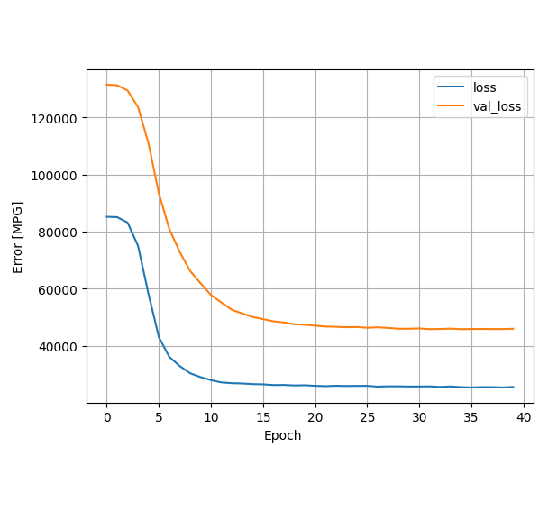
I trained the model for 40 epochs using 10% of the data for validation. The loss metric was mean absolute error, a natural choice for regression tasks like salary prediction where errors are better understood in actual currency terms.
history = dnn_model.fit(
    train_dataset.drop('SALARY', axis=1),
    train_dataset['SALARY'],
    validation_split=0.10,
    epochs=40,
    verbose=1)
dnn_model.save('salary_dnn_model_.h5')
To visualize the training progress, I plotted the training and validation losses across epochs.
def plot_loss(history):
    plt.plot(history.history['loss'], label='loss')
    plt.plot(history.history['val_loss'], label='val_loss')
    plt.xlabel('Epoch')
    plt.ylabel('Error')
    plt.legend()
    plt.grid(True)
plot_loss(history)
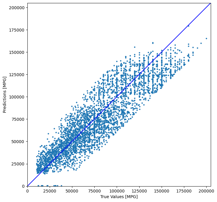
The test results showed that predictions closely followed the actual salaries with most deviations under $20,000. This was a promising outcome for me while dealing with such a human influenced target variable like salary. The finally developed machine learning model was able to predict the salaries of ~4,600 software engineers across 46 countries and 22 job titles (listed at the end of this article) with an average absolute error of approximately USD 20,000 annually.
Interpreting the Results
I examined the prediction errors and grouped them into bins to better understand performance across different ranges. Most errors were small, though high salary roles exhibited higher variance.
prediction_errors = np.abs(test_labels - test_predictions)
error_bins = [0, 10000, 20000, 30000, 40000, 50000, 200000]
bin_labels = np.digitize(prediction_errors, error_bins)
Among these ~4,600 test samples (4584 to be exact), around 1,551 samples (data points) were predicted with an average error of about $10,000 only. Here is the complete distribution:
Prediction Output:
Total test Samples: 4584
- Error range $0 to $10,000: 1551 samples
- Error range $10,000 to $20,000: 1121 samples
- Error range $20,000 to $30,000: 667 samples
- Error range $30,000 to $40,000: 445 samples
- Error range $40,000 to $50,000: 301 samples
- Error range $50,000 to $200,000: 499 samples
Visualizing predicted vs actual salaries confirmed that the model captured the general salary distribution quite well.
plt.figure(figsize=(8, 8))
plt.scatter(test_labels, test_predictions, s=5)
plt.xlabel('True Salaries')
plt.ylabel('Predicted Salaries')
lims = [0, 205000]
plt.xlim(lims)
plt.ylim(lims)
plt.plot(lims, lims, color='b')
Lessons Learned
Data balance is key
Grouping by country and job title helped ensure the model did not overfit to one dominant region or role, which improved fairness.
Encoding shapes the outcome
One hot encoding for high cardinality features like job title allowed the model to learn unique patterns without implying order.
Simplicity and interpretability
Even with a simple 4 layer model, I found that careful preprocessing and normalization mattered more than making the network deeper.
Conclusion
Predicting salaries with deep learning is an exciting blend of curiosity, data craftsmanship, and model intuition. The project taught me that while neural networks can find patterns in human economic data, the real value lies in how we prepare, clean, and interpret that data.
I hope this story inspires you to experiment with structured data modeling, because every dataset has a story to tell, and every model is a way of listening more closely.
💬 Feedback & Support
Loved the app? Have suggestions? Found a bug?
- Blog: analyticalman.com
- Live App: app.analyticalman.com/salary
- Issues: Open a GitHub issue
- Contact: analyticalman.com
Acknowledgments
- Stack Overflow for their comprehensive annual developer survey
- AIJobs.net for providing salary data for Machine Learning Engineers
- The open-source community for amazing ML libraries and tools
If this project helped you, consider giving it a ⭐ on GitHub!
Appendix
All input features along with their unique values are listed below.

